El Niño; El Niño Southern Oscillation; internal waves; trade winds; Kelvin Waves; Rossby Waves; La Nina; Peru Current

El Niño is a warm, nutrient poor, ocean current that flows southward along the coast of northern Peru [Academic American Ency., 1994] and creates sometimes catastrophic effects on local and sometimes global fishing and biogeochemical systems. This event, named El Niño (the {Christ} Child) because it occurs around Christmas time, was once thought of as happening only abnormally. It is known now, however, that El Niño is actually the result of a Pacific Ocean oriented cycle that lasts from three to five years. The event itself lasts about 12 to 18 months.

The El Niño or, more precisely, the El Niño Southern Oscillation (ENSO), for which it and its related phenomena are called, is produced primarily by the interaction between the winds in the atmosphere and the sea surface in the Pacific Ocean. This interaction is tracked by observing, through remote satellites, the changing patterns of sea surface temperatures in the Pacific, sea level changes, and pressure oscillations.

In 1904, Sir Gilbert Walker, Director General of the Observatory in India, began studying the sea level pressure swing between the East Pacific and the West Pacific. He correlated the swing with data from around the globe, including sea surface temperature, and called it the Southern Oscillation (the change in pressure is called the Southern Oscillation Index -SOI- today). Walker failed to make the connection between this oscillation and El Niño however.

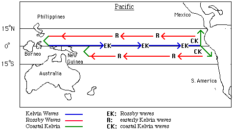
Normally, when there is no El Niño (often referred to as La Niña [Willam H. Schlesinger, 1991]), the trade winds (winds that flow toward the equator) blow from east to west across the coastal waters of the eastern Pacific. In doing so, they drag the warm surface waters of the equatorial Pacific with them. This causes an upwelling of cooler, nutrient-rich waters which the fish population in the region depends on. This 'air/sea interaction' is accompanied by the circulation of large internal waves (waves that have their peaks under the ocean surface) across the Pacific ocean mainly in the equatorial region. These internal waves are referred to as Kelvin and Rossby waves. Kelvin waves travel eastward along the equator and are not subjected to the Coriolis force because of this. Rossby waves, unlike Kelvin waves, travel westward and are a result of the changes that the Kelvin waves introduced to the area. Rossby waves, since they move away, but parallel, to the equator are not relieved of the Coriolis force; thus they travel up to about three times slower.

During an El Niño, the east-to-west trade winds weaken causing the upwelling of deep water to cease. The prevailing reason for this is that cumulus clouds, produced by the warm surface waters of the Pacific, move eastward along the Pacific altering the surface winds and weakening the prevailing east-to-west trade winds. [NASA facts: El Niño, 1994] As the trade winds weaken and the ocean surface is warmed, the El Niño is strengthened and a positive feedback loop forms.

The ENSO cycle can also be explained through the movement of waves in the Pacific as mentioned above. The cycle starts with warm water traveling from the western Pacific to the eastern Pacific in the form of Kelvin waves. After roughly three to four months [Edward Laws, 1992] of traveling across the Pacific along the equator, the Kelvin waves reach the western coast of South America where they mix with the cool Peru Current system; therefore raising sea levels and sealevel temperatures in the region. Upon reaching the coast, the water forks to the north and south and causes El Niño conditions to the south.Because of the changes in sea-level and sea-temperature due to the Kelvin waves, an infinite amount of Rossby waves are formed and move back over the Pacific. The Rossby waves, as mentioned before, are much slower than the Kelvin waves and can take anywhere from nine months to four years [Edward Laws, 1992] to cross the Pacific.Waves move slower when the distance from the equator is increased. (This wave delay is key to the ENSO cycle.) When the Rossby waves arrive at the western Pacific they bounce off the coast and become Kelvin waves and again travel back across the Pacific towards South America. This time, however, the waves decrease the sea-level and sea surface temperature returning the area to normal or La Nina conditions.

This sea surface temperature (SST) oscillation is accompanied by an oscillation in pressure (called the Southern Oscillation). During an El Niño, sea level pressure in the east becomes real low while pressure in the rest rises. The situation reverses itself during La Niña years.

This 3 to 5 year cycle is then repeated and each El Niño phase is different, some being mild and some being very strong. A complete ENSO cycle requires that the Pacific be crossed by two pairs of Kelvin and Rossby waves. Because of El Niño's devastation to local and sometimes global economies and agriculture, the benefits of being able to predict an El Niño even a short while in advance are great.

The El Niño sea surface temperature anomaly is a result of the ENSO cycle. Since the ENSO cycle is produced by a set pattern of ocean and air dynamics in the equatorial Pacific, the sea surface temperature anomaly can be modeled over time and thus an El Niño itself can be predicted.

Although the disastrous effects of El Niño are obvious, the subtle environmental processes that help create it are not. There are several main processes that contribute to the ENSO cycle in the Pacific. These include the Coriolis force, Walker Cell circulation (which produces the trade winds), Meridional cell circulation, and the Southern Oscillation.

The Coriolis force, as mentioned before, effects the traversing of the Kelvin and Rossby waves in the Pacific Ocean. Because of the Earth's rotation, it appears to an observer on Earth that a force is always pushing the wind to the right of the direction of motion in the Northern hemisphere and to the left in the Southern Hemisphere [Laws, E. A., 1992]. To better understand this force, imagine traveling north or south from the equator. As your distance from the equator increases, the circumference of the earth decreases. This causes an exaggeration of the Earth's rotation under an object which moves independently of the Earth itself. The direction of the Earth's rotation thus causes the shift to the right in the Northern Hemisphere and to the left in the Southern Hemisphere. In the case of the internal waves traveling over the pacific in the ENSO cycle, the Kelvin waves move in the relative direction of the Coriolis force (which effectively moves to the right, or towards South America). The Rossby waves, however, must move against this prevailing west-to-east motion and thus travel much more slowly.

The trade winds are caused by a cycle called Walker cell circulation. Waters in the western Pacific are much warmer than those in the east. The warmer air over waters in the west is consequently less dense than the air over waters in the east. As a result, by convection, the western air moves across the Pacific, losing altitude as it slowly cools. Lower air moving from the east to the west, on the other hand, rises when it is heated by the warmer eastern shores. Thus, these disparate temperatures cause a circulation of air which produce the trade winds. El Niño, however, changes that.

Another factor that must first be explained concerning the wind patterns in the Pacific (and elsewhere on the planet) is Meridional cell circulation. Although air tends to rise near the equator, as it moves poleward it radiates heat into outer space and eventually cools and sinks at about 30 degrees latitude. Similarly, cold air that sinks at the poles tends to be warmed as it flows along the surface of the Earth toward the equator and begins to rise near 60 degrees latitude.[Laws, E. A., 1992]

Given this knowledge, we can discuss the trade winds. First, understand that winds are named after the direction from which they are coming, not that in which they are going. The 'westerlies' in the Northern and Southern Hemispheres, therefore, flow from the west because of deflection from the rotation of the earth (which is rotating eastward). The tricky ones are the Northeast and Southeast trade winds. As the Earth's circumference decreases, the eastward rotation becomes slower. Moving north or south will give apparent eastward movement because of this slower rotation.

When El Niño brings its warmer waters to the South American coast, it raises the air temperature. In so doing, it brings the temperature of the east about even with that of the west. Consequently, there is nothing to fuel Walker cell circulation, and the trade winds decline dramatically. The absence of a greater pressure difference also means that warmer waters can stay on the coast. As a result, this part of the ENSO cycle serves as positive feedback by encouraging the prevailing El Niño (or lack there of) conditions.

El Niño causes severe drops in the populations of many animals: turtles, birds, fish, and most specifically, the anchovy. The fishing industry in Peru is extremely dependent on the anchovy, and the livelihood of thousands depends on them. The reduction of the anchovy population, lasting as long as El Niño , that is, up to 18 months, is a terrible blow to this community.

Anchovies live in a specific temperature, and the warm waters of El Niño are too hot for them. The warm, stagnate water does not allow the nutrients which the anchovies thrive on to reach the surface. Whether these conditions kill them or merely force them to move elsewhere is unknown; however, there is no major increase in the anchovy population off the coast of Chile in El Niño years. The anchovy, in fact, might merely dive deeper. The result either way is the same; the anchovies are unreachable to the fishermen's purse seine nets. The warm waters further increase the anchovy's woes by extending the environmental niche of their chief predator, the horse mackerel, which prefers the temperature and is able to come closer to shore.

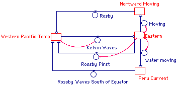
In order to attempt to model and predict the ENSO cycle, the multitude of variables connected with El Niño must first be simplified to a manageable size for the technology available. This report makes use of STELLA II* modeling software (Macintosh version) for both qualitative and quantitative modeling. As a first step, a simple qualitative model was made describing the flow of water/heat by the internal Kelvin and Rossby waves through the Pacific Ocean. Although this model provides a simple dynamical overview of the wave cycle within ENSO, it does little to illustrate what actually goes on during an ENSO cycle.

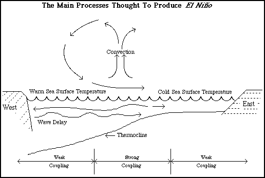
Whereas the major ENSO-related wind changes occur in the central equatorial Pacific, the SST changes occur in the east (which correspond to El Niño/La Niña conditions). The surface wind amplitude depends on the east-west temperature gradient in the Pacific and this corresponds to the temperature variations in the east. The eastern SST is controlled primarily by the oscillation of the thermocline depth. When the SST in the east is warm (and the thermocline is high), the wind anomaly will be westerly, forcing a Kelvin wave 'packet' in the ocean to further depress the thermocline and support current conditions. This area of warm water is compensated by a region of cold water in the form of equatorial Rossby waves moving west. When they reach the west coasts of the Pacific, they are reflected in the form of cool Kelvin waves which move eastward, eventually lowering the SST there. This process takes time, however, and by the time the cool Kelvins are powerful enough to effect the eastern SST, the region has already been significantly warmed (in other words, El Niño has begun). This wave delay is the culprit behind the 'flip-flop' of warm and cold states in the eastern Pacific. [Mark Cane, 1992]

In producing a qualitative model of the ENSO cycle capable of being quantitized, this general description of the ENSO cycle must first be modified for the limitations inherent in STELLA II and transferred to the program. The finished qualitative model is shown below.

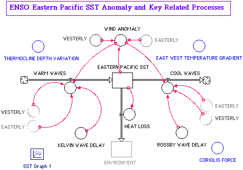
The model above was designed to measure the variation in the sea surface temperature (SST) in the eastern Pacific. It is a dynamical model based on the mathematics of the wave delay mechanism inherent in the ENSO cycle. The model describes the flow of heat in and out of the eastern Pacific region and the main processes controlling it as described above.

The EASTERN PACIFIC SST "reservoir" in the center of the model measures the temperature change in the region over time. It has a single input "flow", WARM WAVES, which heats it. The real world counterpart of WARM WAVES is the warm Kelvin waves which initialize the El Niño event. Its value is determined by the three "converters" attached to it. The purpose of the first two, WESTERLY and EASTERLY, is to tell the WARM WAVES converter whether the winds are 'pushing' the Kelvin waves towards the east (westerlies) or are not (easterlies). The WIND ANOMALY converter decides if the winds are westerly or easterly by a simple if-then relationship:

(IF(Eastern_Pacific_SST>0) THEN(WESTERLY) ELSE(EASTERLY) with EASTERN PACIFIC SST.

The wind anomaly is dependant on SST. EASTERN PACIFIC SST simply records variations in sea surface temperatures and not actual temperatures, therefore numbers above 0 are arbitrarily assigned to be 'warm' temps. and numbers under 0 are assigned to be 'cool' temps. The WARM WAVES flow uses its dependent converters to determine when to send warm water to the EASTERN PACIFIC SST reservoir and how much to send by the equation: IF(WIND_ANOMALY=WESTERLY) THEN(IF(KELVIN_WAVE_DELAY=1) THEN(WESTERLY) ELSE(EASTERLY)) ELSE(0). KELVIN WAVE DELAY is used to calculate the amount of time Kelvin and Rossby waves must travel before they reach the eastern Pacific and will be described in greater detail later.

EASTERN PACIFIC SST also has two output flows, HEAT LOSS and COOL WAVES. HEAT LOSS is a constant flow correlated with the heat that the sea surface temperature loses to the air, land, etc. (ENVIRONMENT) which is eventually radiated away into space. COOL WAVES illustrates the second set of 'cool' Kelvin waves that end an El Niño. Although the model makes it look like the waves are moving warm water away from the eastern Pacific (and thus cooling it), in reality, the waves are cool themselves and flow into the region.

EASTERLY and WESTERLY are used the same way as in WARM WATERS: IF(WIND_ANOMALY=WESTERLY) THEN(IF(ROSSBY_WAVE_DELAY=1) THEN(WESTERLY) ELSE(EASTERLY)) ELSE(0). If the winds are currently westerly (the SST is warm), then the flow will wait a certain amount of time and then begin to cool EASTERN PACIFIC SST thus ending a warm event. Otherwise, they won't do anything (because the SST is already cool and warm waves are getting ready to start a new El Niño).

The wave delay mechanism in the model is key to the mimicking of the ENSO. STELLA II modeling software, unfortunately, has no simple means for making a "flow" wait a certain amount of time before it begins (necessary for the wave delay to function). A round-about alternative, therefore, had to be constructed. After exploring what functions STELLA did provide, a combination of STOPTIME (a STELLA inherent function) and COSWAVE (a simple cosine wave capable of being set to any amplitude difference and period), STOPTIME AND COSWAVE(amp,period), was found to jump back and forth to specified values at specified intervals. With a little reworking of the "flow" equations, they became capable of taking advantage of this feature.

First, consider the COOL WAVES flow. After the warm Kelvin waves begin a warm event, his flow must wait 12 to 18 months (1 to 1.5 years) corresponding to the time it takes the cool waves to start affecting the region. This delay was accomplished by having the ROSSBY WAVE DELAY (STOPTIME AND COSWAVE) function move from 0 to 1 at intervals randomized between 1 and 1.5 (there is no way of knowing exactly how long internal waves will take to cross the Pacific): STOPTIME AND COSWAVE(1,RANDOM(1,1.5)). The original flow equation only starts when ROSSBY WAVE DELAY equals 1 :

IF(WIND_ANOMALY=WESTERLY) THEN(IF(ROSSBY_WAVE_DELAY=1) THEN(WESTERLY) ELSE(EASTERLY)) ELSE(0). This process gives some control over wave cycle.

The WARM WAVES flow, unlike the COOL WAVES flow, has a longer time to wait (assuming that waters in the east are 'cool'). Corresponding to the irregular (but roughly every three to five year) cycle of El Niño events, the WARM WATERS flow, on the beginning of a cool (La Niño) event, waits a randomized 3 to 5 years and then begins to warm the eastern Pacific again. The flow function again is: IF(WIND_ANOMALY=WESTERLY) THEN(IF(KELVIN_WAVE_DELAY=1) THEN(WESTERLY) ELSE(EASTERLY)) ELSE(0).

The converters CORIOLIS FORCE, THERMOCLINE DEPTH VARIATION, and EAST WEST TEMPERATURE GRADIENT are merely included to show what effects the processes included in the mathematical model. They are not included in the mathematical model because of the unnecessary complexity they would introduce and because of a lack of data concerning their affect on the ENSO cycle (specifically the CORIOLIS FORCE). Moreover, from the history of other scientist's attempts at modeling the ENSO cycle, the simple model usually provided the most predictive power.

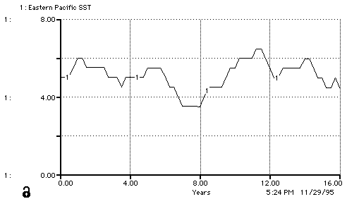
The output of the model was surprising considering the improvisation that had to be done to balance the limitations of the software used. Dismissing the many abrupt changes and watching the basic trends, the output of the model plausibly mimics the oscillations in sea surface temperature in the eastern Pacific. It is very similar to the graph of the SST in the eastern Pacific from the years 1968 to 1984 shown below:

[Edward Laws, 1992, p. 37]

The STELLA model's output corresponds to the variations in eastern Pacific sea surface temperature over time. To verify that the model's output is plausible, the output must 1) be within the range of normal El Niño/La Niña cycles and 2) correspond to the normal occurrences of El Niño events. To accomplish this, SST from an El Niño year will have to be compared to SST in a non-El Niño year to find a typical (preferably max) temperature difference between the two. Additionally, an accurate record of the SST anomaly in the east for a reasonable time period will have to be compared to the model's results to prove the effectiveness of the model in recreating the mechanical processes of the ENSO cycle. This has already been done in the previous section.

SST data in the South Eastern Pacific was obtained from the NASA Jet Propulsion Laboratory Physical Oceanography Distributed Active Archive Center (JPL_PODAAC). The data came on CD-ROM (it's also available over the internet at: ftp://daac.gsfc.nasa.gov/data/inter_disc/surf_temp/). The CD used (Volume V) contained NOAA AVHRR (Advanced Very High Resolution Radiometer) SST data: Monthly Derived Distributions of Satellite-Derived Sea Surface Temperature in HDF format. HDF is a public domain file format specification (developed at the National Center for Super Computing Applications - NCSA) for storing data and images.

In order to find the maximum range of SST in an El Niño event, SST from a very strong EL Niño can be compared to normal (cool) conditions. Fortunately, the greatest El Niño (in heat) in this century occurred in 1982 and a multitude of accurate data was gathered on it. The SST data for this 1982 event (on the PODAAC CD), as said before, comes in AVHRR HDF data sets. The HDF files contain pixel color values (digital numbers) corresponding to SST in the South Eastern Pacific (23.5deg.N to 66.5deg.S Longitude and 159.0deg.W to 69.0deg.W Latitude). In order to convert this pixel color value into actual SST values in degrees Celsius, a simple macro must be run on each of the data points in the data file:

SST = .15*Pixel_Color_Value - 2.1 [http://http://www.nadn.navy.mil:80/Oceanography/MIDS/SO486/SO486_project.html]

The two images that follow are the original pixel color value image and the resulting actual SST image from the December 1982 El Niño conditions in the South East Pacific (off South America).

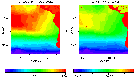
The two data images appear so dissimilar because their respective scales have different color distributions and different units (pixel colors vs. Celsius degrees). Neither image has the warm water 'triangle' off the coast of Peru characteristic of El Niño. One must remember that the SST oscillation associated with El Niño is relatively small and will not appear in images of global sea surface temperatures. By subtracting normal, La Niña sea surface temperatures from these El Niño sea surface temperatures, however, the temperature anomaly can be emphasized. Using SPYGLASS TRANSFORM, SST from the 304 day of 1983 was subtracted from the SST values of the 304 day of 1982. The macro that did this simply subtracted each data point value in the '83 data set from its counterpart in the '82 data set. The following images show the results in two different color scales (for effect).

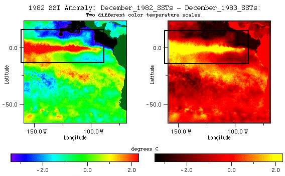
The SST anomaly is now very prominent (in the rectangular box). From the images, it appears that the El Niño region is roughly 2 and 1/4 degrees Celsius higher than the 'normal' temperatures. If the SSTs never changed between the two years, then all the data points on these graphs would be zero (or light green in the left image). These data verify the model's output range of approximately 2deg. to -2deg. C. (See Modeling section above)

ENSO modeling began from a base of useful hypotheses as to the mechanisms governing ENSO [Mark Cane, 1992]. The early models had little data to work with and none that was conclusive. These models have evolved into comprehensive Global Climate Models (GCMs) that must be run on a supercomputer for output. During the process, several "in-between" models were created which, although being simple, provided recognizable simulations of ENSO and had some predictive power. The difficulty in producing realistic output even in the most state-of-the-art GCMs for the ENSO cycle has pushed the limits of the climate modeling capabilities now in existence. Several of these models have achieved success in predicting SST anomalies even a year in advance. It has been found that the more general models which produce basic trends instead of trying to account for everything, often have the best results (and are also cheaper to run). The following set of model outputs is from the NINO3 model.

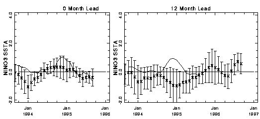
Forecasts of NINO3 SST Anomalies: Results are presented for two different lead times ranging from 0 months to 12 months. Each forecast is actually the mean of forecasts from six consecutive months, adjusted to have the same mean and standard deviation as the observed. Note that 0 month lead can differ from the observed because SST data is not used in initialization. For each lead time, forecast values are indicated by x's and observed values by a solid line (for 12 month lead times, observed values are 3 month averages; otherwise they are monthly averages). Error bars represent root-mean-square error, based on the years 1972-1987.These indices are calculated by averaging SST Anomaly field over the NINO3 area (which is in the eastern equatorial Pacific).

The model has several drawbacks. Although its output is within range (both in temperature and duration), it doesn't predict what will happen, only what could happen. The model relies only on the dynamics of the wave motion in the Pacific (including their reliance on the wind anomaly). It leaves out minute wind variations, pressure, sea level, and numerous other processes which effect the ENSO. Moreover, because of the limitations of the STELLA II software, the wave delay mechanism in the model is not very reliable.

The modeling section discussed the steps which were taken to balance STELLA's inability to wait or pause a "flow" when an IF-THEN statement becomes true. In order for the wave delay to function, the COOL WAVES flow must wait 12 to 18 months after the eastern Pacific becomes warm before its cool waves start to return the region to normal conditions. STOPTIME and COSWAVE were used to count off this duration, jumping from 1 to 0 every 12 to 18 months. The COOL WAVES "flow" starts when the waters in the eastern Pacific are warm and when ROSSBY WAVE DELAY = 1. The problem is that, since ROSSBY WAVE DELAY is a separate function running on its own, it could be 1 exactly when COOL WAVES judges how long it has to wait (by reading WAVE DELAY's value). In this case, there would be no delay. This is not necessarily a bad thing; the resulting El Niño would just be very short. This, however, wouldn't be consistent with the time it takes the internal waves to traverse the Pacific. So, in conclusion, the time interval could be greater or less than the 3 to 5 year scale because of the limitations of the method used to model the wave delay.

The last and most significant problem with the model is that it doesn't rely on actual data to make its predictions. The model is entirely mathematical with only one link to what actually is going on in the Pacific. Each time the model is run, one can decide the initial value of the eastern Pacific SST. The only data that is included in the current model is whether the eastern Pacific SST is warm or cool, and this is arbitrary depending on the year the model starts.

Future generations of this model would include the CORIOLIS FORCE, THERMOCLINE DEPTH VARIATION, and EAST WEST TEMPERATURE GRADIENT as data inputs. Also, the relationship between SST, pressure (Southern Oscillation), and sea level would be made more prominent considering that the three anomalies occur at the same time and affect one another. Although the current model has significant limitations, it does produce a plausible ENSO cycle SST oscillation which corresponds to the actual time scales of El Niño/La Niña events.

1 - Cane, Mark. Climate System Modeling: "Tropical Pacific ENSO models: ENSO as a mode of the coupled system", Cambridge University Press, NY, NY, 1992

2 - El Niño; Academic American Encyclopedia. PRODIGY interactive personal service, (C)1994 Groiler Electronic Publishing, Inc.

3 - El Niño and Climate Prediction. Reports to the Nation (http://www.pmel.noaa.gov/toga-tao/el-nino-report.html)

4 - Glantz, M. Teleconnection Linking Worldwide Climate Anomalies. Cambridge University Press, NY, NY, 1991

5 - Laws, E. A. El Niño and the Peruvian Anchovy Fishery. Oceanography Department, University of Hawaii, Honolulu, 1992.

6 - Monastersky, Richard. Old and tired, an El Niño hints of its end. July 4, 1992 SCIENCE NEWS

7 - Monastersky, Richard. The Long View of Weather, Learning how to read the climate several seasons in advance. March 20, 1993, SCIENCE NEWS Vol. 144

8 - Monastersky, Richard. Two decades of Pacific warmth have fired up the globe. March 11, 1995, SCIENCE NEWS Vol.147

9- NASA Facts. El Niño. Goddard Space Flight Center. The Mission to Planet Earth Series, February 1994.

10 - Tran, Andy. Satellite-Derived Multichannel Sea Surface Temperature and Phytoplankton Pigment Concentration Data: PODAAC, JPL, January 30, 1993.

11 - Schlesinger, Willam H. Biogeochemical Analysis of Global Change; . Academic Press INC. (C) 1991.

12 - SPYGLASS TRANSFORM Quick Reference Guide, Version 3.0, 1993

13- STELLA II Technical Manual, High Performance Systems, 1990

14 - Tighe, Tahan, Berhane, Davis. El Nino (http://www.circles.org/ESSCC/curric/reports/gzag/93_94/el_nino/1stWelcomtoElNino.html]